
What we plan to cover in this blog is listed below
- Transformations
- Rotations
- Scaling
- Image Pyramids
- Cropping
- Convolutions and BLuring
- Sharpening
- Thresholding and Binarization
- Edge Detection and Image Gradients
Transformations
Transformations are distortions enacted upon an image. What we can do with these transformations, we use them to correct distortions or perspective issues from arising from the point of view an image was captured.
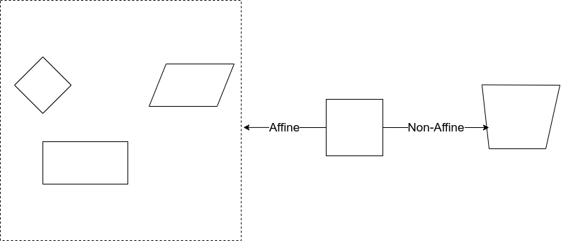
There are two types of well-known transformation one is affine and the other one is Non-Affine.
Affine Vs Non-Affine
Affine transformations include things such as scaling, rotation and translation. The important factor is if the lines are parallel in the original image then after transformation also, lines will be in parallel. What I said in simple words parallelism between lines also be maintained after the transformation also.
In Non-Affine transform, parallelism will not be maintained. The non-affine transform does not preserve Parallelism, length, and angle. It does, however, preserve collinearity and incidence.
Rotations
Rotations, You know that. A rotating image is easy. We can rotate about a point and this point commonly is the centre of an image. How we can do a rotation with OpenCV will look below. For rotation, we have M matrix which is given below
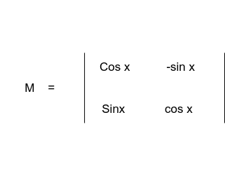
The angle is measured anticlockwise from the horizontal line which is drawn from the centre.
OpenCV allows you to scale and rotate at the same thing using the function which is called getRotationMatrix2D.
Arguments of getRotationMatrix2D functions are a point where we need to rotate( in our case, the centre point ), angle of rotation(90 anticlockwise) and the scale(1) factor.
iamge = cv2imread(iamge_path)
height, width = iamge.shape[:2]
#Center point is (width/2, height/2)
rotatation_matrix = cv2.getRotationMatrix2D((width/2, height/2),90,1)
rotated_image = cv2.warpAffine(image, rotation_matrix, (width,height))
cv2.imshow('Rotated Image', rotated_iamge)
cv2.waitKey(0)
cv2.destroyAllWindows()
Resizing or Scaling
It is very simple but Here, we need to care about one thing that is interpolation. what is interpolation? simply, It is a method of constructing new data points within the range of a discrete set of known data points. Basically, when we do resize it means we are expanding the points or pixels. How can we find the gaps between the pixels when we are resizing an image from big to small or small to big? We do interpolation to fill the gap of pixels.
OpenCV has many types of interpolations.
cv2.INTER_AREA → Good for shrinking or downsampling
cv2.INTER_NEAREST → Fastest
cv2.INTER_LINEAR → Good for zooming or upsampling(default)
cv2.INTER_CUBIC → Better
cv2.INTER_LANCZOS4 → Best
image = cv2.imread(image_path)
image_scaled_default = cv2.resize(image, None, fx=0.75, fy =0.75)
cv2.imshow('Scaling Default', image_scaled_default)
img_scaled_cubic = cv2.resize(image, None,fx =2, fy=2, interpolation = cv2.INTERCUBIC)
cv2.imshow('Scaling Cubic Interpolation', img_scaled_cubic)
img_scaled = cv2.resize(image, (800,600), interpolation = cv2.INTER_AREA)
cv2.imshow("scaling - exact size", img_scaled)
cv2.waitKey(0)
cv2.destroyAllWindows()
cv2.resize function can be used to resize the image. we can scale the image with a ratio(fx, fy) of the original image like the first two scaling examples.
We can set the exact size to scale the image like the last example.
Cropping
Cropping is very easy in OpenCV. images are represented as Numpy arrays in openCV. So we can use that to crop the images. When we know the exact four coordinates where we need to crop, We can use Numpy array method
cropped = image[x1:x2, y1:y2]
Here x1 and x2 are the row coordinates and y1 and y2 are column coordinates.
Convolutions(*) and Blurring
Convolution is a mathematical operation performed on two functions producing a third function which is typically a modified version of one of the other original functions
Output image = Image * Function(Kernal size)
In computer vision, we use kernel’s to specify the size over which we run our manipulating function over our image.
Convolution basically operates one by one pixel at a time. So when the convolution operates at a pixel it will consider the around the pixels which are included in the kernel. Convolution looks at the values of kernel pixels then operates each pixel at a time.
Blurring is an operation where we average the pixels within a region(kernel).
cv2.filter2D is the basic blurring method in OpenCV
We define a kernel which is 3 x 3 like below
              | 1 1 1 |
kernel = 1/9 *| 1 1 1 |
              | 1 1 1 |
We multiply by 1/9 to normalize otherwise we would be increasing intensity. When we divide by 9 the sum will be as 1.
img = cv2.imread(image_path)
kernel = np.ones((3,3), np.float32)/9
blurred_img = cv2.filter(img, -1, kernel)
When we increase the kernel size then the blurring will be high.
There are other blurring functions also in OpenCV such as box blurring and Gaussian blurring.
The box filter is an average filter. this takes the pixels under the box and replaces the central element. so the box size needs to an odd and positive number. Below is a method to use the box filter in opencv
blur_img = cv2.blur(img, (3,3))
medianBlur is another blur filter that is taking median instead of the average.
median = cv2.medianBlur(img,5)
The bilateral filter is very effective in noise removal while keeping edges sharp. It also takes a Gaussian filter in space, but one more Gaussian filter which is a function of pixel difference. The pixel difference function makes sure only those pixels with similar intensity to the central pixel is considered for blurring. So it preserves the edges since pixels at edges will have large intensity variation.
bilateral_img = cv2.bilateralFilter(img, 9, 75, 75)
GaussianBlur Filter is another filter that is using the Gaussian matrix. Gaussian matrix has different weights instead of the same number. The Gaussian kernel has a peak value in the centre and slows down to the corner.
guassian_img = cv2.GuassianBlur(img, (7,7),0)
Image De-noising-Non-Local-Means Denoising filter is different from the above-mentioned filters. This filter actually originates from computational photography methods. It takes some time to run.
flitered_img = cv2.fastNlMeanDenoisingColored(image, None, 6,6,7,21)
Sharpening
Sharpening is the opposite of blurring. It strengthens or emphasizing edges in an image.
sharpening_kernel = np.array([[-1,-1,-1],
                              [-1,9,-1],
                              [-1,-1,-1]
                              ])
sharped_img = cv2.filter2D(img, -1,sharpening_kerne)
Our kernel sum is equal to one so we don’t need to normalize again.
Thresholding AND Binarization
Thresholding is the act of converting an image into a binary form. All threshold types are applied to grayscale images.
cv2.threshold(image, Threshold value, Max value, Threshold type)
ret, thresh = cv2.threshold(image, 127,255,cv2.THRESH_BINARY)
When we use the above function values below 127 goes to 0 and other values will be 255
ret, thresh = cv2.threshold(image, 127,255,cv2.THRESH_BINARY_INV)
When we use the above function values below 127 goes to 255 and others are zero.
ret, thresh = cv2.threshold(image, 127,255,cv2.THRESH_TRUNC)
When we use above function values above 127 are truncated at 127( the 255 argument is unused)
ret, thresh = cv2.threshold(image, 127,255,cv2.THRESH_TOZERO)
when the above function is called, values below 127 go to 0 above 127 are unchanged.
ret, thresh = cv2.threshold(image, 127,255,cv2.THRESH_TOZERO_INV)
when the above function is used, below 127 is unchanged, above 127 goes to 0.
thresh = cv2.adaptiveThreshold(image, 255, cv2.ADAPTIVE_THRESH_MEAN_C, cv2.THRESH_BINARY,3,5)
Above function, we have used an adaptive threshold.
thresh_vl, thresh_img = cv2.threshold(image, 0,255,cv2.THRESH_BINARY+cv2.THRESH_OTSU)
A simple threshold or global threshold requires us to provide a threshold value. Adaptive threshold methods take that uncertainty away.
cv2.adaptiveThreshold(image, Max Value, Adaptive Type, Thresold Type, Block size, Constant that is subtracted from mean)
Here, Block size should be an odd number.
Adaptive threshold types
1. ADAPTIVE_THRESH_MEAN_C → Based on the mean of the neighborhood of pixels
2. ADAPTIVE_THRESH_GAUSSIAN_C → weighted sum of neighborhood pixels under Gaussian kernel
3. THRESH_OTSU → Clever Algorithm assumes there are two peaks in the grayscale histogram of the image and then tries to find an optimal value to separate those peaks to find T.
Edge detection
Edges are not only the boundary of images but also sudden changes in an image also can be an edge.
Edges can be defined as sudden changes in an image and they can encode just as much information as pixels.
OpenCV has three main types of Edge Detection algorithms
- Sobel → To emphasize vertical or horizontal edges
- Laplacian → Gets all orientations
- Canny → Optimal due to low error rate, well-defined edges and accurate detection.
Canny is an excellent edge algorithm to detect the edges. It was developed by John F.Canny in 1986
Steps of Canny Edges Detection
- Applies Gaussian Blurring
- Finds intensity gradient of the image
- Applied non-maximum suppression(Removing the pixels which are not edges)
- Hysteresis — Applies thresholds(If the pixel is within the upper and lower thresholds it is considered as an edge)
sobel_x = cv2.Sobel(img, cv2.CV_64F, 0,1,ksize =5)
sobel_y = cv2.Sobel(img, cv2.CV_64F, 1,0,ksize =5)
Sobel can detect the horizontal and vertical edges separately.
Canny Edge detection takes only two threshold values to detect the edges. Any gradient value larger than thresh_high is considered to be an edge. Any value below threshold_low values considered not to be an edge. Values in between the threshold values are either classified as edges or non=edges based on how their intensities are connected.
edges_detection = cv2.Canny(img,thresh_low, thresh_high)


0 Comments