
Sorry to disappoint but no- I am not referencing WWE superstar Edge but rather the edges of an image used online. This is an important topic as — when programmers are trying to search or identify objects in an image — finding the border or edge of the image is very important. This article will look at the fundamentals of edges with the main focus on various methods for edge detection.
What is an edge?
Essentially an edge is a discontinuity representing changes in an image attribute (for example, luminance and texture are both important primitive features). If we scan an image along a horizontal line and draw a profile of colour, we can observe a change of colour along the edge. (in this example the background and foreground colours are different). This particular change is the change that you can see in the continuity of this colour level. These kinds of changes are referred to as edges, and they can appear to be incredibly sharp (also known as a “sudden manner”) or gradual (known as “gradients”). This article will look into some of the fundamental techniques that can be used to find the gradients and/or enhance them.
Let’s Dig into the fundamentals of edge detection
Since edges are the results of gradients (or some other class of image attributes), we need to identify the gradients.
For an image function f(x,y), we can define two gradients x and y-direction respectively. The gradient at any point can be defined as:
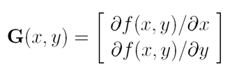
The direction of the gradient vector G at (x,y) (measured with respect to the x-axis) is:
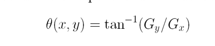
where
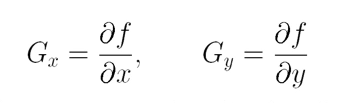
The gradient vector points in the direction of the maximum rate of change of f at the location (x,y).
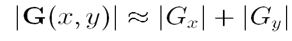
So for edge detection, we are interested in the magnitude of the gradient.
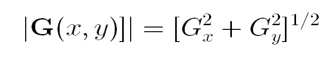
But practically, we will not carry out the above calculation since this is computational demand. We often go with the approximation function which can indicate the gradient change.
The above gradient theory can be applied to images as we will get a matrix of pixel values instead of functions. One approach for this is using two-point approximations.
The two-point approach
In this approach, we take one pixel and then another pixel from the next direction. Next, we observe the intensity difference between these two and — based on whether there is a difference or not- see whether there is a gradient.
| 20 21 80 20 30 34|
| 32 23 43 34 34 34|
| 34 34 34 45 56 56|
Let’s look at the pixel value 43. When we calculate the partial derivate in the x-direction (34–43)/1 the result is -9 (as the next pixel value is 34 and we take delta x as 1-pixel distance).
For the y-direction, (80–43)/1 = 37
We can do the same with the convolution function with the help of the following masks.
In the x-direction, we can use |-1 +1| mask and,
in the y-direction, we can use:
|+1|
| -1 |
Since the current pixel becomes minus, and the next pixel becomes plus, the convolution operation will work. We take two pixels and find the gradient however, please note that if any noise occurs then our gradient will fail. So, how do we handle this situation? Well, we need something more complex than a two-point approach. This is what we call a three-point approach
The three-point approach
| 20 21 80 20 30 34|
| 32 23 43 34 34 34|
| 34 34 34 45 56 56|
Here, we consider three pixels. For the particular pixel(43) in the x-direction, we take the left(23) and right(34) pixels. We consider the difference(23–34 = 11) between right and left pixels rather than the middle one. If there is a gradient, we can see the difference between left and right.
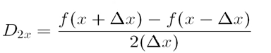
Here, we can ignore the scaling factor 2 ( 2 pixels) for easy computation.
Similarly to the x-direction, in regards to the y-direction the gradient of y will be (80–34) = 47
For the convolution mask, we can define it as follows:
x-direction mask |-1 0 +1|
y-direction mask
|+1|
|+0|
| -1 |
Even if we use this approach, our noise problem will be present so rather than taking 3 pixels we consider 3 rows of pixels.
| 20 21 80 20 30 34|
| 32 23 43 34 34 34|
| 34 34 34 45 56 56|
For value 43, we do gradient above row 43, at row 43, and below row 43.
Above → (20–21) = -1
At → (23–34) = -11
Below →(34–45) =-11
Then we average it to get the x-direction gradient of 43 pixel = (-1 + -11 +-11) = -7.6667
We can do the same for y-direction as below
((21–34) +(80-34) + (20-45))/3 = 3
When we carry out the above, we consider 9 pixels meaning that the noise of one pixel will be negated.
With the above intuition, we can define the masks of the:
X-direction
|-1 +0 +1|
|-1 +0 +1|
|-1 +0 +1|
Y-direction
|+1 +1 +1|
|+0 +0 +0|
|-1 - 1 -1|
These two masks are called Prewitt masks.
The Sobel operator for edge detection
The X-direction Kernel of Sobel is the same as the x-direction Prewitt mask with weighted values for the same row of pixels, as such:
|-1 +0 +1|
|-2 +0 +2|
|-1 +0 +1|
Y-direction Kernel of Sobel
|+ 1 + 2 + 1|
|+ 0 + 0 + 0|
| — 1 — 2 — 1|
X-direction edges will be determined by Y- direction gradients and vice versa.
Look at the below image to understand the edge detection based on gradient direction.
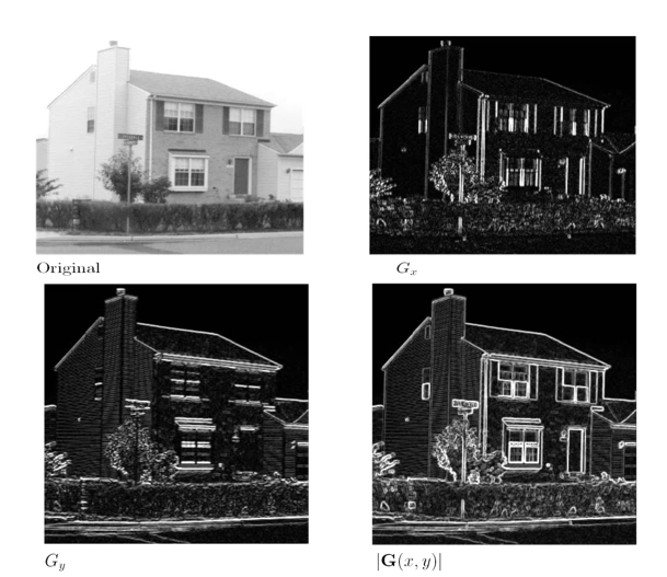
If you look ar Gx, you can see that it will be used to detect the Y direction edges and if you look at Gy it will use to detect the X direction edges. Using G(x,y) to detect both x directions and y directions edges.
Using the Correct Threshold to detect edges
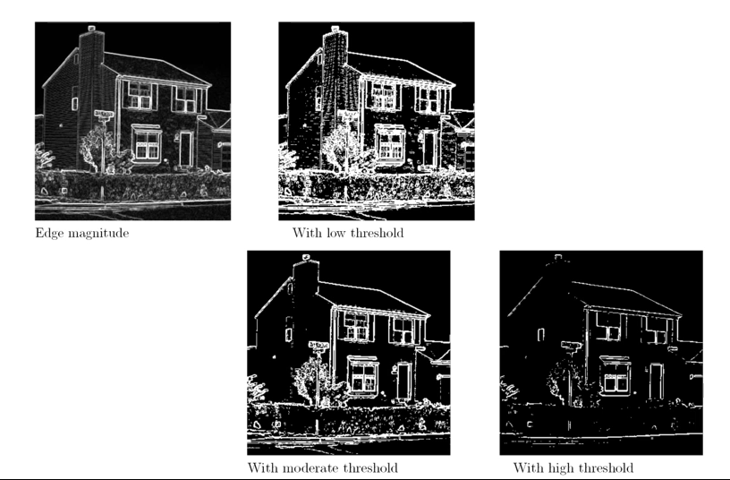
When we apply a low threshold for gradients to filter out that time, we see some of the edges that are not what we were interested in and also presented in the detection. When we apply a high threshold for gradients to filter out that time, we can miss some edges that are we interested in. The threshold value is playing a vital role in the edges of the image that are presented.
Let’s Look at the Practical scenario
In most cases, we will not get a clear or ideal image. Instead, we will get a noisy image and we need to detect the edges from that image. When we apply the standard edge detection to noisy images we will be misled by the noise. So when we do edge detection, we will do a noise removal preprocessing before the detection.
One way to do this is by carrying out a mean filter to remove Gaussian noise which has the added benefit of smoothing out edges as well. Using the Laplacian operator, which can give the second derivative of the pixel. The second derivative will be zero when the first derivate is in maximum and also the first derivate is zero.
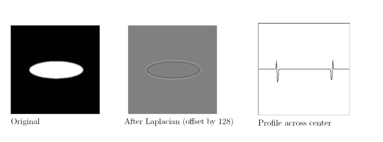
Based on the above, the Laplacian operator is seldom used by itself for edge detection because it is unacceptably sensitive to noise. However, it is useful in determining whether a given pixel is on the dark or light side of an image. Often this operated is used in conjunction with a Gaussian filter for edge detection known as a Laplacian of Gaussian filter. With this laplacian, we can find the edge easily as at the edge it will give zero. Here’s the process:
- First, we apply a very large filter to remove the noise
- Using the Laplacian operator we find the edges
Laplacian + Gaussian filters are linear meaning that we can apply both filters in a single run to reduce computational power.
Canny Edge detection
An easy to follow tutorial on how to build a Canny edge detector algorithm explained step by step.towardsdatascience.com
Read the above article to understand canny edge detection.
Conclusion
Being able to detect an image’s edges is a very helpful and often useful skill for developers. This article ran through a number of methods to achieve just this, I hope it has been helpful! Thanks for reading and please leave any feedback or questions in the comments. Happy detecting!


0 Comments